A couple of posts back I wrote about discovering Elevation Profiles for Paths in Google Earth. I’ve spent a little bit more time working with this, and came up with another neat activity for a classroom.
In the last post I created a path with only two endpoints – basically a straight-line cross section. I also did this across fairly large areas of land, entire states, in fact. This activity focuses in on the details a bit, and uses the directions section of Google Earth.
First, go to the Directions tab and input two locations. These can be addresses, lat-long coordinates, or any other type of locator. For this activity, I suggest keeping the distances fairly short, probably within about 50 miles. Here are some suggestions:
- From your home to your school, workplace, or church
- Between two cities
- Between your house and your best friend’s house
In the example below, I used Greenville and Spartanburg.
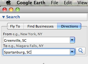
When you hit Enter or click on the magnifying glass search icon, you get driving directions between the two cities. For some strange reason Google Earth chose Wade Hampton Boulevard instead of I-85. I guess it went with the shortest route rather than the quickest. No matter – I can still illustrate the point.
Once the route and directions are generated, you should see the path icon at the bottom of the driving instructions. You can right-click on that path to get the elevation profile between those two points. You may want to click to embiggen the image.
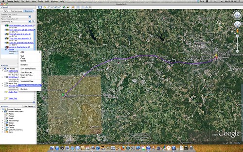
Bear in mind that the elevation profile tends to be exaggerated, especially if you’re generating one for a relatively short distance. Even though it’s exaggerated, you can see the high and low points of the route.
Looking at the elevation profile, imagine the route as you might travel it. Could you envision the high points and low points? What geographical features might match those points?
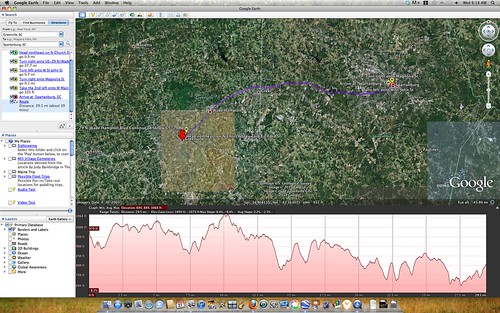
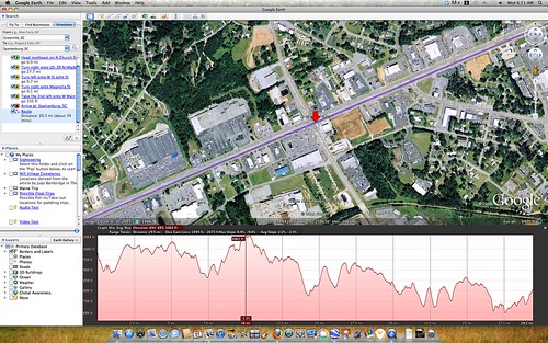
On the Greenville to Spartanburg route I moved the red pointer so that it was on one of the lower dips about mid-way in the profile. I clicked on the elevation profile to center the map on that point, then used the page up key to zoom into that location.
The image below shows that this is where the South Tyger River crosses Wade Hampton. Many of these dips are associated with rivers and streams, but that’s not always the case.
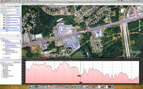
But what about the peaks? The exaggerated nature of the profile would make one think that we’re climbing Alps here, but that’s just not the case. When I zoomed to the highest point on the profile it just looks like an ordinary intersection, nothing special. I know from driving that area that it does go downhill in both directions from that point. I just hadn’t realized how high that spot was until I saw the profile.
There are other questions that could be asked about an elevation profile. For example, which city is higher above sea level? The profile clearly shows Greenville much higher than Spartanburg by a whopping 168 feet. (OK, so it’s really not THAT much.)
You can also ask about the maximum elevation change, from highest point to lowest. In this case, the highest point is 1064 ft. above sea level at the intersection of Wade Hampton and Highway 290, and the lowest is at 688 ft. where E. O. Ezell Boulevard crosses a small stream near downtown Spartanburg. The maximum elevation change is 376 ft.
Assuming that it takes less fuel to go uphill than down, could students use elevation profiles to plot an alternate route that might be more fuel efficient? Would there be a distance vs elevation formula that could be used to make the calculations? I could think of lots of activities along these lines.